Lab4: Segmentation
Introduction
Three levels of image analysis:
- Classification: Given an image $x$ and return as output a class $y = f_\theta(x)$.
- Object detection: Given an image $x$, identify meaningful object inside of it, draw a rectangle that specify its position and classify each indetified object.
- Segmentation: Given an image $x$, classify each pixel of $x$ into one possible class.
This is generally done with a Convolutional Neural Network that act as an image-to-image transform, mapping each pixel of $x$ to the corresponding class.
Remind: Given an image $x \in \mathbb{R}^{m \times n \times c}$, an image-to-image map is a function $f: \mathbb{R}^{m \times n \times c} \to \mathbb{R}^{m' \times n' \times c'}$. In our situation, $m = m'$, $n = n'$ and $c = c'$. An image-to-image map is required to do segmentation and some image processing tasks, but not for classification or object detection. \
Image-to-image maps are usually implemented by some variant of a Fully Convolutional Neural Network (FNN) design (e.g. ResNet, Autoencoders, ...). See https://heartbeat.comet.ml/a-2019-guide-to-semantic-segmentation-ca8242f5a7fc for details.
Dataset: Carvana Image Masking Challenge
In our experiments today, we will use a famous dataset for image segmentation, which is called Carvana (https://www.kaggle.com/competitions/carvana-image-masking-challenge/overview). We need to download it:
- Login with you kaggle account on https://www.kaggle.com/ .
- Go to the link of the challenge and subscribe to the rules of the challenge.
- In Account, press Create New API Token. This will download a file named $\texttt{kaggle.json}$. Upload this file on Colab.
- Run the following.
# Install Kaggle library
!pip install kaggle

# Create a new folder .kaggle and move kaggle.json into that
!mkdir ~/.kaggle
!mv kaggle.json ~/.kaggle/

# Allocate permissions for this file
!chmod 600 ~/.kaggle/kaggle.json
# Download the data from the competition. If an error occours, either you did
# something wrong on the above or you forgot to subscribe the challenge.
!kaggle competitions download -c carvana-image-masking-challenge
# The dataset is huge. For our experiments today, we just need a subset of it.
# Unzip train.zip and the corresponding masks. Not the HQ version.
!unzip -p carvana-image-masking-challenge.zip train.zip >train.zip
!unzip -p carvana-image-masking-challenge.zip train_masks.zip >train_masks.zip

# Unzip the zipped train files.
!unzip train.zip
!unzip train_masks.zip
Setup
Import libraries and prepare the code.
# Utilities
import os

# Algebra
import numpy as np

# Visualization
import matplotlib.pyplot as plt
from PIL import Image
import cv2

# Neural Networks
import tensorflow as tf
from tensorflow import keras as ks
def load_data_from_names(root_dir: str, fnames: list, shape=(256, 256)) -> np.array:
    # Given the root path and a list of file names as input, return the dataset
    # array.
    images = []

    for idx, img_name in enumerate(fnames):
        x = Image.open(os.path.join(root_dir, img_name))
        x = x.resize(shape)
        x = np.array(x)
        images.append(x)

        if idx%100 == 99:
            print(f"Processed {idx+1} images.")
    return np.array(images)

# Load the names
image_names = os.listdir('./train')
mask_names = os.listdir('./train_masks')

image_names.sort()
mask_names.sort()

# To reduce the computational time, we consider only a subset of the dataset
N = 2000 # Number of total datapoints

image_names = image_names[:N]
mask_names = mask_names[:N]

# Create data. We will always use the notation that "x" is the input of the
# network, "y" is the output.
x = load_data_from_names('./train', image_names)
y = load_data_from_names('./train_masks', mask_names)

# Print the dimension of the dataset.
print(f"The dimension of the dataset is: {x.shape}")
# Split the training set into training and test.
TRAIN_SIZE = 1800

x_train = x[:TRAIN_SIZE]
y_train = y[:TRAIN_SIZE]

x_test = x[TRAIN_SIZE:]
y_test = y[TRAIN_SIZE:]

print(f"Train size: {x_train.shape}. Test size: {x_test.shape}")
Train size: (1800, 256, 256, 3). Test size: (200, 256, 256, 3)
Visualization
Visualize some image and the corresponding mask.
def show(x, y, title=None):
    plt.figure(figsize=(15, 8))

    plt.subplot(1, 2, 1)
    plt.imshow(x)
    if title:
        plt.title(title[0])

    plt.subplot(1, 2, 2)
    plt.imshow(y)
    if title:
        plt.title(title[1])

    plt.show()

show(x_train[0], y_train[0])
Model
def build_cnn(input_shape, n_ch, L=3):
    x = ks.layers.Input(shape=input_shape)

    h = x
    for i in range(L):
        h = ks.layers.Conv2D(n_ch, kernel_size=3, padding='same')(h)
        h = ks.layers.ReLU()(h)

        n_ch = 2*n_ch

    y = ks.layers.Conv2D(1, kernel_size=1, activation='sigmoid')(h)
    return ks.models.Model(x, y)

CNN_model = build_cnn((256, 256, 3), 64, L=3)
CNN_model.compile(optimizer=ks.optimizers.Adam(learning_rate=1e-4),
                  loss='binary_crossentropy',
                  metrics=['accuracy'])

print(CNN_model.summary())
# Set hyperparameters
BATCH_SIZE = 16
N_EPOCHS = 20

# Training
hist = CNN_model.fit(x_train, y_train,
              batch_size=BATCH_SIZE,
              epochs=N_EPOCHS,
              validation_split=0.1)

# Check overfit
loss_history = hist.history['loss']
val_loss_history = hist.history['val_loss']

acc_history = hist.history['accuracy']
val_acc_history = hist.history['val_accuracy']

plt.plot(loss_history)
plt.plot(val_loss_history)
plt.grid()
plt.xlabel('Epoch')
plt.legend(['Loss', 'Val Loss'])
plt.title('Loss')
plt.show()

plt.plot(acc_history)
plt.plot(val_acc_history)
plt.grid()
plt.xlabel('Epoch')
plt.legend(['Accuracy', 'Val Accuracy'])
plt.title('Accuracy')
plt.show()
Evaluation
There are multiple metrics used to measure the quality of the segmentation. The most important are:
- Accuracy
- Intersection over Union (IoU)
- Dice Coefficient
Accuracy
The accuracy is simply defined by considering the segmentation as a pixel-by-pixel classification. \
Intersection over Union
The Intersection over Union (IoU) is pretty intuitive. It is defined as the ratio between the intersection area between the predicted mask and the ground truth mask, over the union between the two masks.
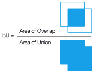
By using that the mask is a binary image, it is trivial to compute both the intersection and the union (the latter, computed via the relationship:
$$ \mu (A \cup B) + \mu (A \cap B) = \mu (A) + \mu (B) $$
where $\mu(A)$ is defined to be the Area of A. \
Clearly, $IoU(y, y') \in [0, 1]$, and $IoU(y, y') = 1$ in the best case, where $y$ and $y'$ overlap perfectly, and $IoU(y, y') = 0$ when they don't overlap.
Dice coefficient
The Dice coefficient is defined by twice the overlapping area of the two masks, over the sum of the area of the two masks.
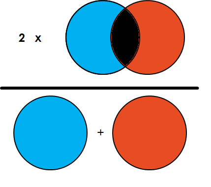
The implementation of the dice coefficient is similar to the implementation of the IoU, since both of them explicitely uses that a mask is between 0 and 1.
from keras import backend as K
from keras.losses import binary_crossentropy

def iou_coeff(y_true, y_pred):
    smooth = 1

    intersection = K.sum(K.abs(y_true * y_pred), axis=[1,2,3])
    union = K.sum(y_true,[1,2,3]) + K.sum(y_pred,[1,2,3]) - intersection

    iou = K.mean((intersection + smooth) / (union + smooth), axis=0)
    return iou

def dice_coeff(y_true, y_pred):
    smooth = 1

    y_true_f = K.flatten(y_true)
    y_pred_f = K.flatten(y_pred)
    intersection = K.sum(y_true_f * y_pred_f)
    score = (2. * intersection + smooth) / (K.sum(y_true_f) + K.sum(y_pred_f) + smooth)
    return score

# Function that evaluate the model on a dataset
def evaluate_model(model, x, y, fun):
    y_pred = model.predict(x) # Use the model to predict the output
    y = np.expand_dims(y, -1) # We need to add the channel dimension on y

    # Uniform the type of the array
    y_pred = y_pred.astype('float32')
    y = y.astype('float32')

    return fun(y, y_pred)

iou = evaluate_model(CNN_model, x_test,  y_test, iou_coeff)
dice = evaluate_model(CNN_model, x_test,  y_test, dice_coeff)

print(f"The IoU of the trained model is {iou}, while its Dice coefficient is {dice}.")
# Qualitative results
y_pred = CNN_model.predict(x_test[:1])

show(x_test[0, :, :], y_test[0, :, :], title='Original')
show(x_test[0, :, :], y_pred[0, :, :, 0], title='Predicted')
UNet
Maybe the most known network architecture used for segmentation is the UNet.
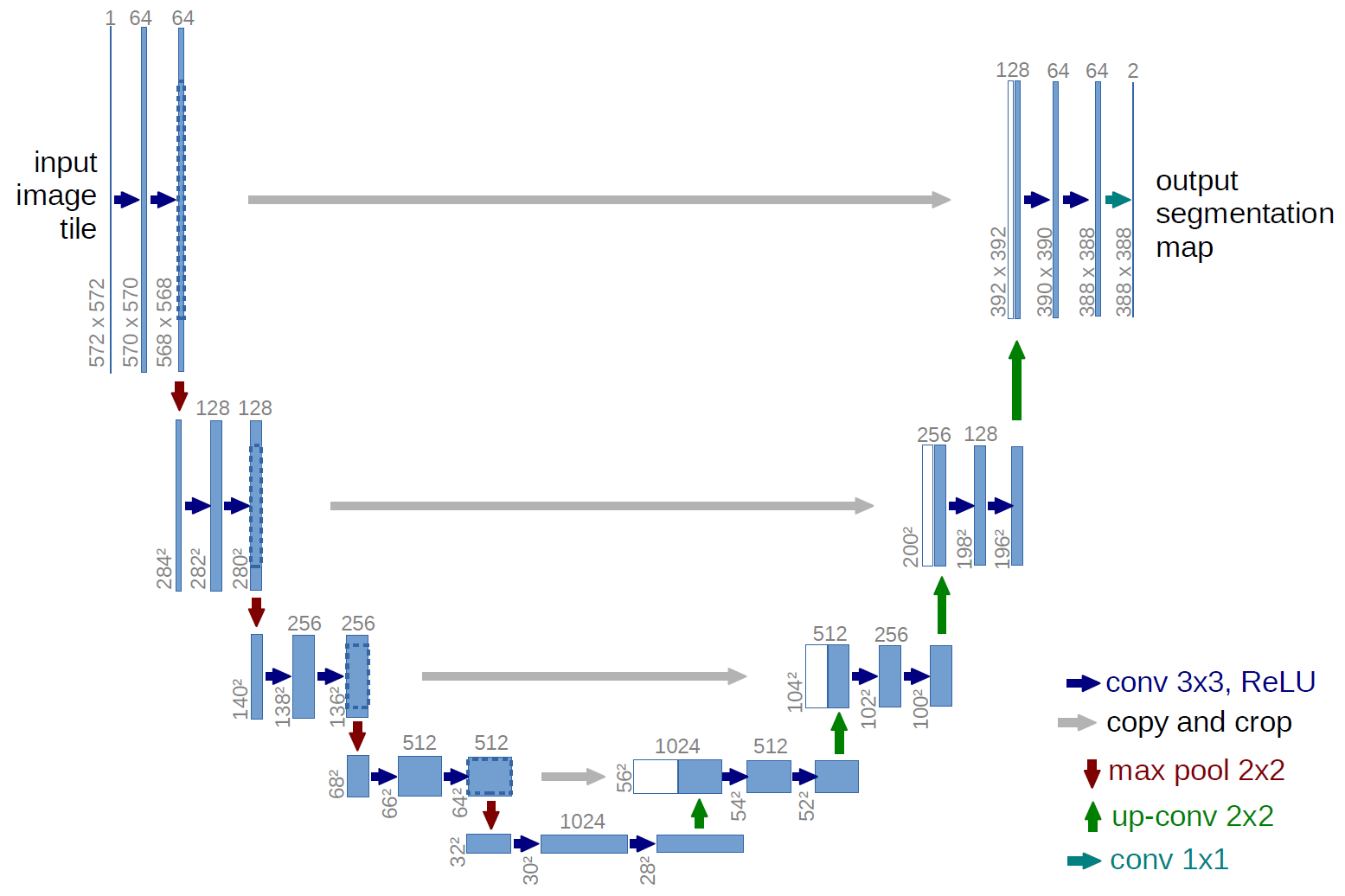
its architecture is based on the formula that you studied to compute the receptive field of a convolutional neural network:
$$ D' = S(D-1) + K $$
where $D'$ is the receptive field of the previous layer, $D$ is the receptive field on the following layer, $S$ is the stride and $K$ is the kernel size. \
A consequence of this formula is that the receptive field increases exponentially while moving down, linearly while moving right. \
The drawback of downsampling, which is the information loss, is solved by UNet by adding skip connections, that also act as training stabilizer. \
Note that, at every downsampling (which in this case is implemented as a MaxPooling2D layer), the number of filters double, to reduce the impact of the dimensionality loss (the total number of pixel after downsampling is divided by 4).
# Exercise: try to implement your version of UNet, based on the diagram above.
#           remember that the initial number of channels must be given as
#           input and it doubles every time you go down.
#           Moreover, it is required that the number of "floors" of the network
#           must be a parameter. The same should happen for the number of each
#           convolution per level.
#
#           Remember that, to go down, you need to use the MaxPooling2D operator
#           while to go up, a strided transpose convolution is required.
#
#
#
#           Train the UNet defined in this way on the dataset above. It performs
#           better or worse?
# Training
BATCH_SIZE = 16
N_EPOCHS = 20

hist = unet_model.fit(x_train, y_train,
              batch_size=BATCH_SIZE,
              epochs=N_EPOCHS,
              validation_split=0.1)
# Check overfit
loss_history = hist.history['loss']
val_loss_history = hist.history['val_loss']

acc_history = hist.history['accuracy']
val_acc_history = hist.history['val_accuracy']

plt.plot(loss_history)
plt.plot(val_loss_history)
plt.grid()
plt.xlabel('Epoch')
plt.legend(['Loss', 'Val Loss'])
plt.title('Loss')
plt.show()

plt.plot(acc_history)
plt.plot(val_acc_history)
plt.grid()
plt.xlabel('Epoch')
plt.legend(['Accuracy', 'Val Accuracy'])
plt.title('Accuracy')
plt.show()
unet_model.save_weights('segmentation_unet_train.h5')
iou = evaluate_model(unet_model, x_test,  y_test, iou_coeff)
dice = evaluate_model(unet_model, x_test,  y_test, dice_coeff)

print(f"The IoU of the trained model is {iou}, while its Dice coefficient is {dice}.")
# Qualitative results
y_pred = unet_model.predict(x_test[:1])

show(x_test[0, :, :], y_test[0, :, :], title='Original')
show(x_test[0, :, :], y_pred[0, :, :, 0], title='Predicted')
Data augmentation
When using a very powerful model (such as UNet) to solve a Segmentation task, there is a chance that your model will overfit. Given a fixed model, overfit happens strongly if the number of datapoints is small. Thus, a way to reduce overfitting is to enlarge the dimension of the dataset. \
This is very easy to do in Segmentation. Given a (sufficiently regular) tranformation $T: \mathbb{R}^{m \times n \times c} \to \mathbb{R}^{m \times n \times c}$ and a dataset $\mathbb{D} = \{ (x_i, y_i) \}_{i=1}^N$, where $x_i$ is an image and $y_i$ is a mask with the same dimension of the corresponding image, we can create a new dataset $\mathbb{D}_{ex} = \{ (\tilde{x}_i, \tilde{y}_i) \}_{i=1}^{2N}$ where $\tilde{x}_i = x_i, \tilde{y}_i = y_i$ for $i = 1, \dots, N$, $\tilde{x}_i = T(x_i), \tilde{y}_i = T(y_i)$ for $i = N+1, \dots, 2N$. \
This procedure can be repeated for multiple transormations $T$, to obtain a larger dataset. \
Warning: Data augmentation via regular transformations $T$ does not add information to the dataset. As a consequence, the training complexity will increase linearly with the number of transformation we apply, without resulting in an improvement on the knowledge the model has. As a consequence, simply using tens of transormations to create a big dataset is not necessary a good idea. I suggest to use at most a couple of them, such as flipping, rotating or shifting.
def apply_transform(x_data, y_data, T):
    N = x_data.shape[0]

    new_x_data = np.zeros_like(x_data)
    new_y_data = np.zeros_like(y_data)

    for i in range(N):
        new_x_data[i] = T(x_data[i])
        new_y_data[i] = T(y_data[i])
    return new_x_data, new_y_data

def augment_data(x_data: np.array, y_data: np.array, transforms: list) -> np.array:
    new_x_data = x_data
    new_y_data = y_data

    for T in transforms:
        new_x, new_y = apply_transform(x_data, y_data, T)

        new_x_data = np.concatenate([new_x_data, new_x], axis=0)
        new_y_data = np.concatenate([new_y_data, new_y], axis=0)
    return new_x_data, new_y_data

# Augment our data with flipud and fliplr
transforms = [np.flipud, np.fliplr]
augmented_x_train, augmented_y_train = augment_data(x_train, y_train, transforms)